Some Practical Examples with Excel Solver

Excel Solver is one of the most useful features you can come across while analyzing data in Excel. This is a what-if analysis feature in the form of an Excel Add-in. This article will focus on different examples of the Solver feature in Excel including many different areas.

What Is Solver in Excel?

Solver is a Microsoft Excel add-in program. The Solver is part of the What-If Analysis tools that we can use in Excel to test different scenarios. We can solve decision-making issues using the Excel tool Solver by finding the most perfect solutions. They also analyze how each possibility impacts the worksheet’s output.

How to Enable Solver Feature in Excel

You can access Solver by choosing Data ➪ Analyze ➪ Solver. Sometimes it may happen that this command isn’t available, you have to install the Solver add-in using the following steps:

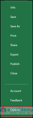
• First of all, choose the File
• Secondly, select Options from the menu.

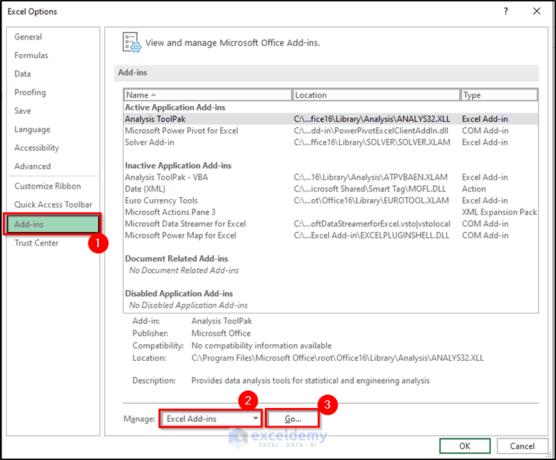
• Thus, the Excel Options dialog box appears.
• Here, go to the Add-Ins
• At the bottom of the Excel Options dialog box, select Excel Add-Ins from the Manage drop-down list and then click Go.

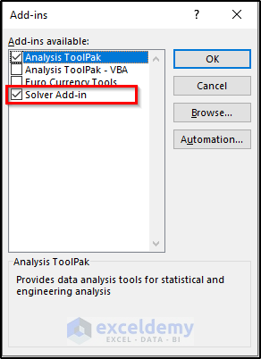
• Immediately, the Add-ins dialog box appears.
• Then, place a checkmark next to Solver Add-In, and then click OK.

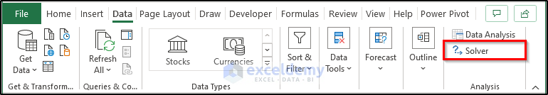
Once you activate the add-ins in your Excel workbook, they will be visible on the ribbon. Just move to the Data tab and you can find the Solver add-in on the Analyze group.

How to Use Solver in Excel

Before going into more detail, here’s the basic procedure for using Solver:

• First of all, set up the worksheet with values and formulas. Make sure that you have formatted cells correctly; for example, the maximum time you can’t produce partial units of your products, so format those cells to contain numbers with no decimal values.
• Next, choose Data ➪ Analysis ➪ Solver. The Solver Parameters dialog box will appear.
• Afterward, specify the target cell. The target cell also is known as the objective.
• Then, specify the range that contains the changing cells.
• Specify the constraints.
• If necessary, change the Solver options.
• Let the Solver solve the problem.

Initially, we are going to focus on two simple problems using the Excel solver. The first one will be maximizing profit from a series of products and the second one focuses on minimizing the production cost. These are just two examples to show the procedure of Excel solver in two different scenarios. More problems regarding the same feature will follow in the later part of the article.

Example 1: Application of Excel Solver to Get Maximize Profit of Products

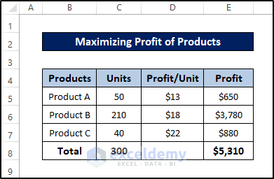
Let’s take a look at the following dataset first.

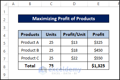
The highest profit comes from Product C. Therefore, to maximize total profit from production, we can produce only Product C. But if things were so straightforward, you wouldn’t need tools like Solver. This company has some constraints that must be met to produce products:

• The combined production capacity is 300 units per day.
• The company needs 50 units of Product A to fill an existing order.
• The company needs 40 units of Product B to fill an expected order.
• The market for Product C is relatively limited. So the company is not interested in producing more than 40 units of this product per day.

Now let’s see how we can use the solver to work with the problem.

Steps:

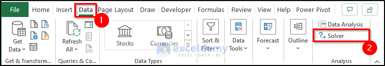
• First, go to the Data tab on your ribbon.
• Then select Solver from the Analysis group.

• Now select cell E8 as the objective cell of the Solver Parameter box.
• Besides the To: options select Max as we are trying the maximize the value of the cell.
• In the By Changing Variable Cells, select the cell values we are mainly focusing on changing. Here, they belong to the range C5:C7.
• Now add the constraints by clicking on the Add button on the right of the box.
• Finally, select Simplex LP in the Select a Solving Method box.

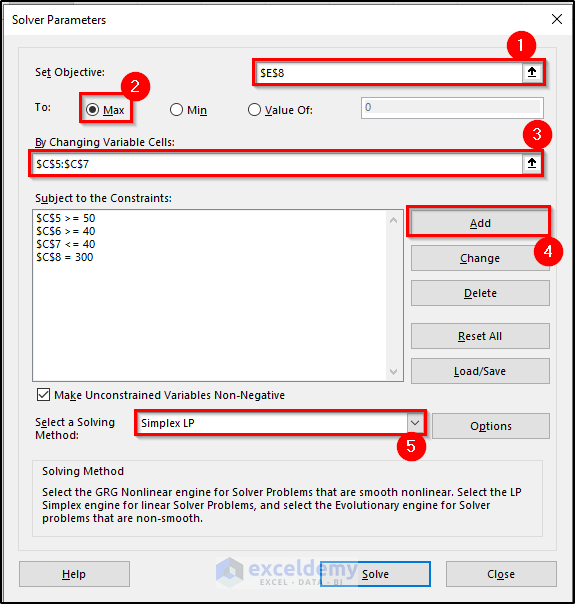
• Once you are done with all the steps above, click on Solve at the bottom of the box.
• After that, the Solver Results box will appear.
• Now select the options and reports you want to prefer in this box. For the demonstration, we are choosing to enable the Keep Solver Solution option only.

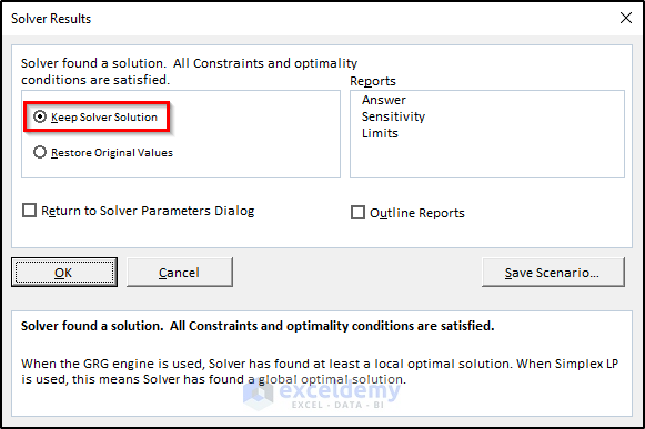
• Next, click on OK.
• The dataset will now change to this.

This indicates the optimum number of units required to have the maximum profit within the constrained entered. This is just one of the examples that demonstrate how powerful the Excel solver feature can be.

Example 2: Use of Excel Solver for Minimizing Shipping Cost

After the maximizing problem above, let’s look at an example focusing on minimizing values. We will use SUM and SUMPRODUCT functions for calculating different parameters. For that, let’s take the following dataset.

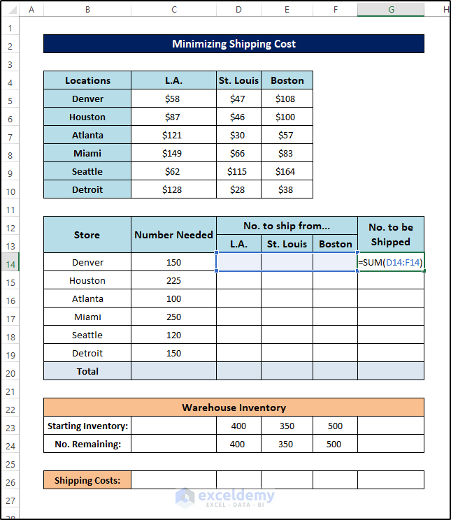
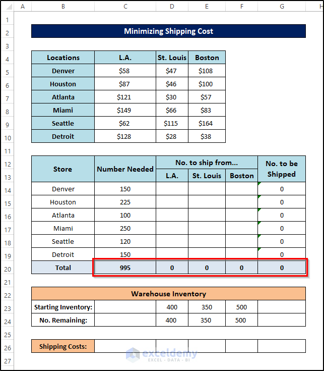
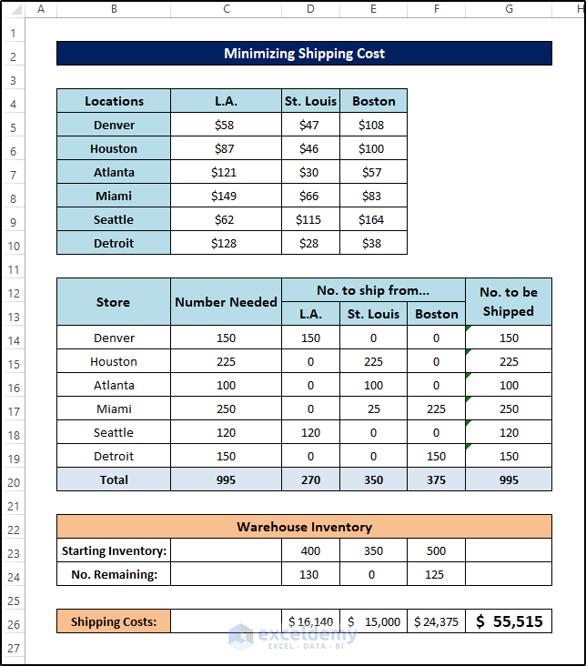
Shipping Costs Table: This table contains the cell range B4:E10. This is a matrix that holds per-unit shipping costs from each warehouse to each retail outlet. For example, the cost to ship a unit of a product from Boston to Detroit is $38.

Product needs of each retail store: This information appears in the cell range C14:C19. For example, the retail outlet in Houston needs 225, Denver needs 150 units, Atlanta needs 100 units, and so on. C18 is a formula cell that calculates the total units needed from the outlets.

No. to ship from…: Cell range D14:F19 holds the adjustable cells. These cell values will be varied by Solver. We have initialized these cells with a value of 25 to give Solver a starting value. Column G contains formulas. This column contains the sum of units the company needs to ship to each retail outlet from the warehouses. For example, G14 shows a value of 75. The company has to send 75 units of products to the Denver outlet from three warehouses.

Warehouse inventory: Row 21 contains the amount of inventory at each warehouse. For example, the Los Angeles warehouse has 400 units of inventory. Row 22 contains formulas that show the remaining inventory after shipping. For example, Los Angeles has shipped 150 (see, row 18) units of products, so it has the remaining 250 (400-150) units of inventory.

Calculated shipping costs: Row 24 contains formulas that calculate the shipping costs.

The solver will fill in the values in the cell range D14:F19 in such a way that will minimize the shipping costs from the warehouses to the outlets. In other words, the solution will minimize the value in cell G24 by adjusting the values of cell range D14:F19 fulfilling the following constraints:

• The number of units demanded by each retail outlet must equal the number shipped. In other words, all the orders will be filled. The following specifications can express these constraints: C14=G14, C16=G16, C18=G18, C15=G15, C17=G17, and C19=G19
• The number of units remaining in each warehouse’s inventory must not be negative. In other words, a warehouse can’t ship more than its inventory. The following constraint shows this: D24>=0, E24>=0, F24>=0.
• The adjustable cells can’t be negative because shipping a negative number of units makes no sense. The Solve Parameters dialog box has a handy option: Make Unconstrained Variables Non-Negative. Make sure this setting is enabled.

Let’s walk through the following steps to do the task.

Steps:

• First of all, we will be setting some necessary formulas. To calculate to be shipped, type the following formula.

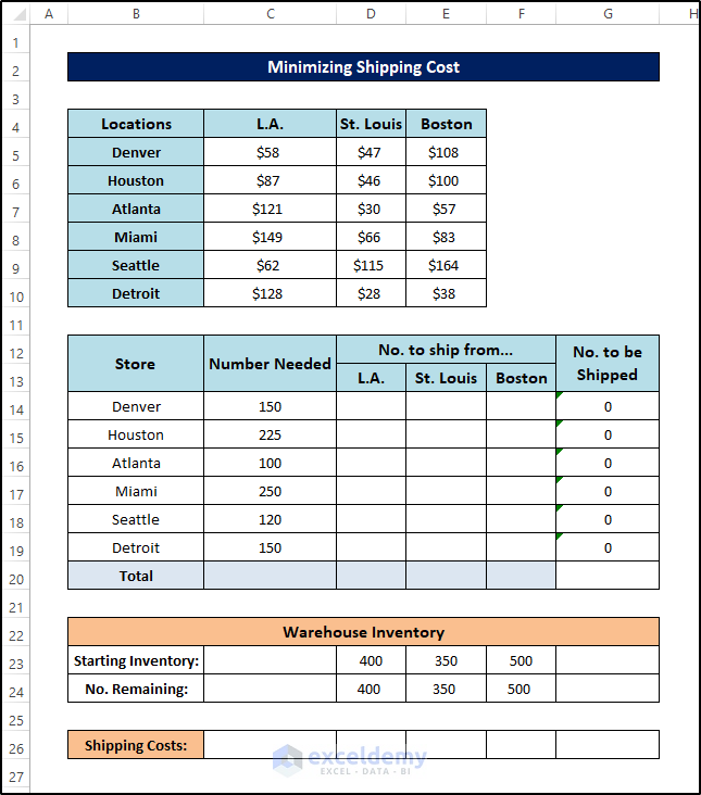
• Then, press Enter.

• Next, drag the Fill Handle icon up to cell G19 to fill the other cells with the formula.
• Therefore, the output will look like this.

• Afterward, to calculate the total, type the following formula.

• Then, press Enter.

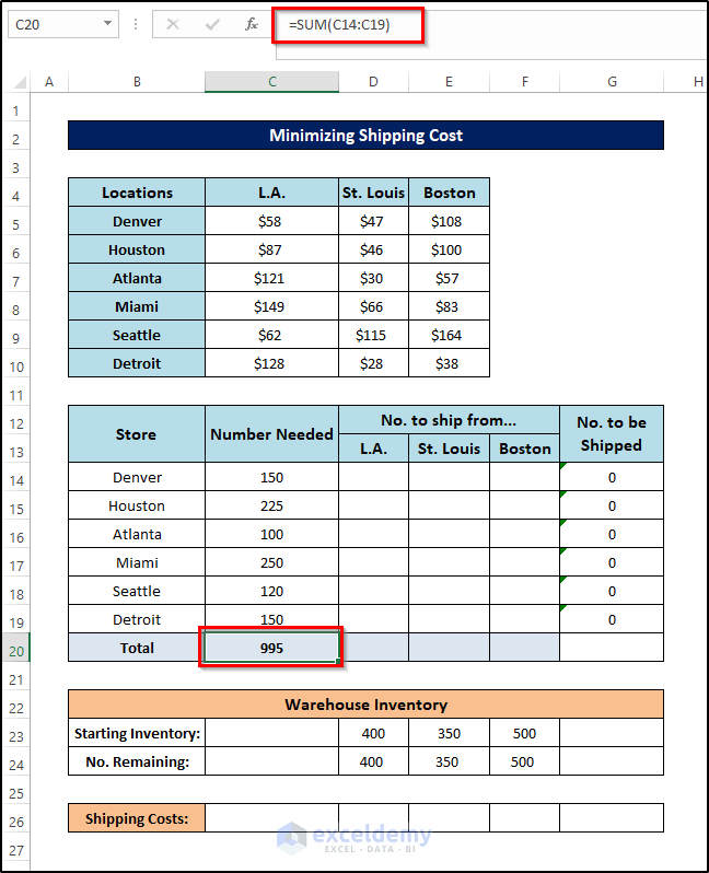
• Next, drag the Fill Handle icon to the right up to cell G20 to fill the other cells with the formula.
• Therefore, the output will look like this.

• Afterward, to calculate the shipping costs, type the following formula.

• Then, press Enter.

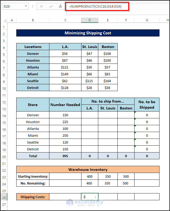
• Next, drag the Fill Handle icon to the right up to cell F26 to fill the other cells with the formula.
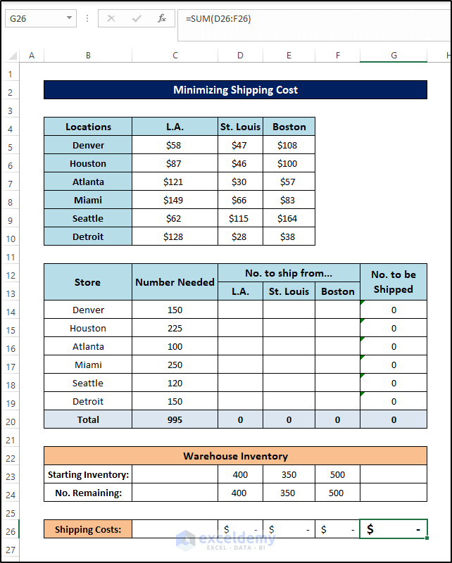
• Now type the following formula in cell G26.

• To open the Solver Add-in, go to the Data tab and click on Solver.

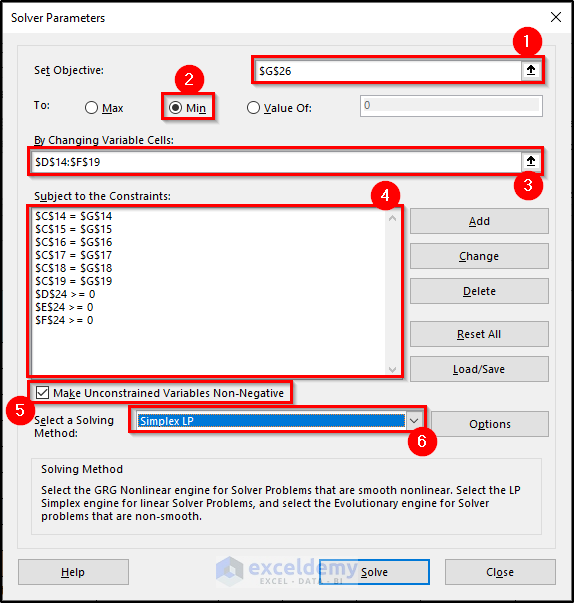
• Next, fill the Set Objective field with this value: $G$26.
• Then, select the radio button of the Min option in To Control.
• Select cell $D$14 to $F$19 to fill the field By Changing Variable Cells. This field will show then $D$14:$F$19.
• Now, Add constraints one by one. The constraints are: C14=G14, C16=G16, C18=G18, C15=G15, C17=G17, C19=G19, D24>=0, E24>=0, and F24>=0. These constraints will be shown in the Subject to the Constraints field.
• Afterward, select the Make Unconstrained Variables Non-Negative check box.
• Finally, select Simplex LP from the Select a Solving Method drop-down list.

• Now, click on the Solve The following figure shows the Solver Results dialog box. Once you click OK, your result will be displayed.

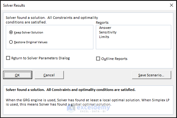
• The Solver displays the solution shown in the following figure.

More About Excel Solver

We’re going to discuss the Solver Options dialog box in this section. Using this dialog box, you can control many aspects of the solution process. You can also load and save model specifications in a worksheet range using this dialog box.

Usually, you’ll want to save a model only when you use more than one set of Solver parameters with your worksheet. Excel saves the first Solver model automatically with your worksheet using hidden names. If you save additional models, Excel stores the information in the form of formulas that correspond to the specifications. (The last cell in the saved range is an array formula that holds the options settings.)

It may happen that Solver will report it can’t find a solution, even when you know that one solution should exist. You can change one or more of the Solver options and try again. When you click the Options button in the Solver Parameters dialog box, the Solver Options dialog box shown in the following figure appears.

A simple Solver example in Excel

We can control many aspects of how Solver will solve a problem.

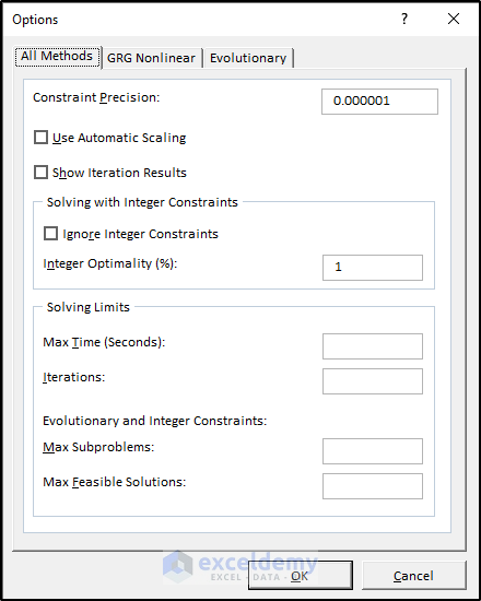
Here is a brief description of Solver’s options:

Constraint Precision: Specify how close the Cell Reference and Constraint formulas must be to satisfy a constraint. Specifying less precision will make Excel solve the problem more quickly.

Use Automatic Scaling: It is used when the problem deals with large differences in magnitude— when you attempt to maximize a percentage, for example, by varying cells that are very large.

Show Iteration Results: By selecting this checkbox, the Solver is instructed to pause and display the results after each iteration.

Ignore Integer Constraints: If you select this check box, Solver will ignore constraints that mention that a particular cell must be an integer. Using this option may permit Solver to find a solution that can’t be found otherwise.

Max Time: Mention the maximum amount of time (in seconds) that you want Solver to spend on a single problem. If the Solver reports that it exceeded the time limit, you can increase the amount of time that it will spend searching for a solution.

Iterations: Enter the maximum number of trial solutions that you want Solver to try to solve the problem.

Max Subproblems: It is used to solve complex problems. Specify the maximum number of sub-problems that may be solved by the Evolutionary algorithm.

Max Feasible Solutions: It is used for complex problems. Specify the maximum number of feasible solutions that may be solved by the Evolutionary algorithm.

Example 3: Investment Portfolio Optimization with Excel Solver

In this section, we will look at an investment portfolio problem, which can also be said to be a financial problem. We are going to optimize such with the help of the Excel solver. The aim of portfolio or financial optimization is to identify the optimal portfolio (asset distribution) among those that are portfolios given a certain objective. In most cases, the objective is to maximize benefits, like predicted return, while minimizing liabilities, such as financial risk.

Let’s look at the following investment portfolio.

The problem statement is described below.

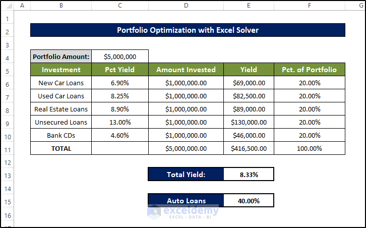
• The amount that the credit union will invest in new-car loans must be at least three times the amount that the credit union will invest in used-car loans. The reason is: that used car loans are riskier investments. This constraint is represented as C5>=C6*3
• Car loans should make up at least 15% of the portfolio. This constraint is represented as D14>=.15
• Unsecured loans should make up no more than 25% of the portfolio. This constraint is represented as E8<=.25
• At least 10% of the portfolio should be in bank CDs. This constraint is represented as E9>=.10
• The total amount invested is $5,000,000.
• All investments should be positive or zero.

Follow these steps to see how you can use the solver in Excel for examples like this.

Steps:

• First, select the Data
• Then select Solver from the Analysis

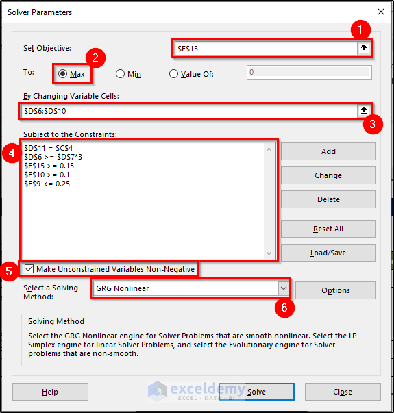
• Now Fill the Set Objective field with this value :$E$13.
• Then select the radio button for the Max option in To
• After that, select cell $D$6 to $D$10 to fill the field By Changing Variable Cells. This field will show then $D$6:$D$10.
• Add constraints one by one. The constraints are: $D$11= $C$4 $D$6>= $D$7*3, $E$15>= 0.15, $F$9<= 0.25, $F$10>= 0.1. These constraints will be shown in the Subject to the Constraints box.
• Select the Make Unconstrained Variables Non-Negative check box.
• Select GRG Nonlinear from the Select a Solving Method drop-down list.

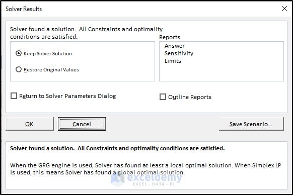
• Now click the Solve Click OK.
• There will be another dialog box in which you need to select the result types.
• This means you need to select Keep Solver Solution. Otherwise, the values will revert back to the original values.
• Then from the right side of the dialog box, select all the options in the Reports.
• Then click OK after this.

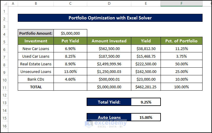
• We’ve entered 1,000,000 in the changing cells as the starting values. When you run Solver with these parameters, it produces the solution shown in the following figure which has a total yield of 25%.
• The Auto Loans values also changed to 15%.
• And this is how we got the highest optimization value of Total Yield considering all the constraints.

And this is how we complete the optimization of an investment portfolio using the Excel solver.

Example 4: Linear Integer Programming Using Excel Solver

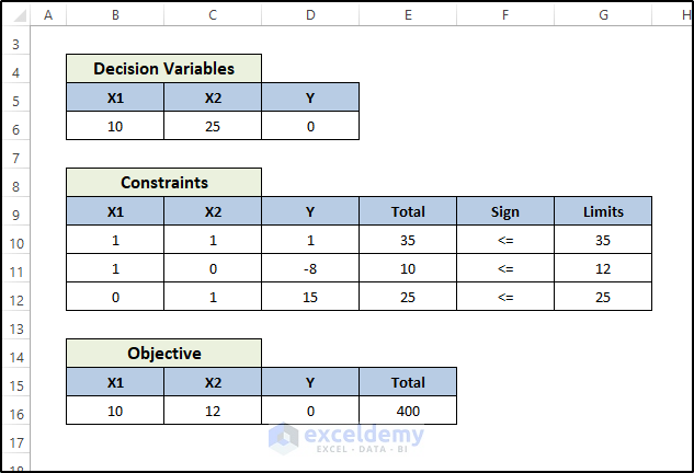
Let’s take a look at an example of an Excel solver’s usage in Integer Linear programming. First, take a look at a suitable dataset for the problem.

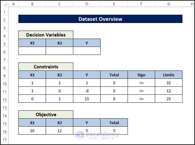
Now it’s time to look at the particulars of the Excel solver for this integer linear programming example:

Now follow these steps to see how we can solve this particular integer linear programming example in Excel using the solver.

Steps:

• First, go to the Data tab and select Solver from the Analysis

• Now put in the values and constraints in the Solver Parameter box as shown in the figure.

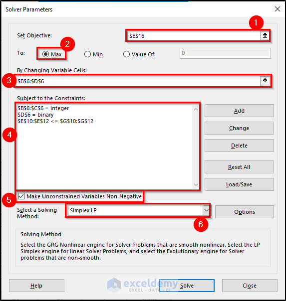
• Then click on Solve.
• Next, click OK on the Solver Results.

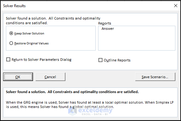
The final result of using the Excel solver on the integer linear programming example will be like this.

Read More:  Example with Excel Solver to Minimize Cost

Example 5: Scheduling with Excel Solver

Suppose that the bank has 22 employees. How should the workers be scheduled so that they would have the maximum number of weekend days off? We will maximize the number of weekend days off with a fixed number of employees in this scheduling example of the Excel solver.

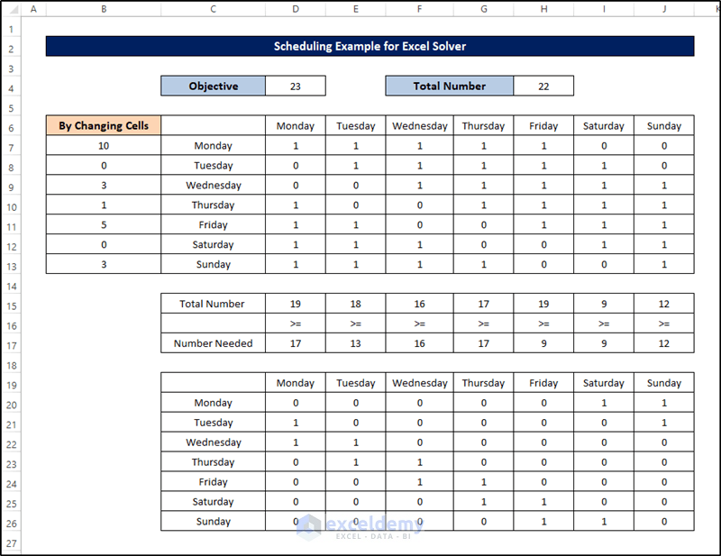
Let’s look at the dataset.

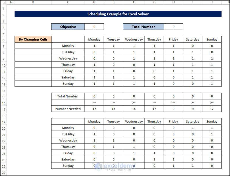
The constraints are shown in the figure. To solve the scheduling problem and use the solver in examples like that you can follow these steps.

Steps:

• First, go to the Data tab on your ribbon and select Solver from the Analysis

• Next, put in the values of the constraints and the parameters as shown in the figure below.

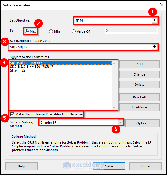
• After that, click on Solve.
• Finally, click on OK on the Solver Results.

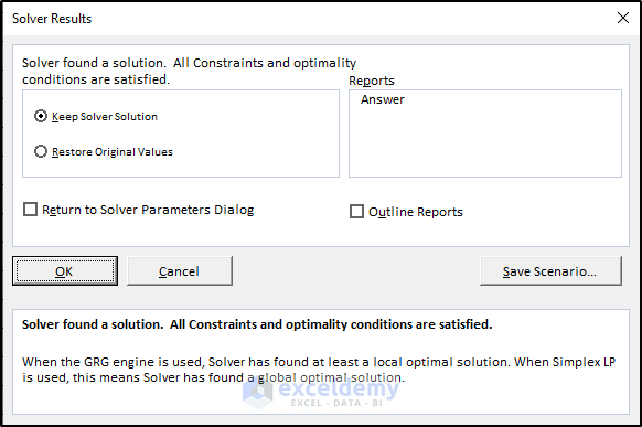
The solver will automatically show the result of the scheduling problem on the Excel spreadsheet because of the choices we made in the steps.

You can use the solver in Excel in similar examples like that.

Read More: How to Assign Work Using Evolutionary Solver in Excel

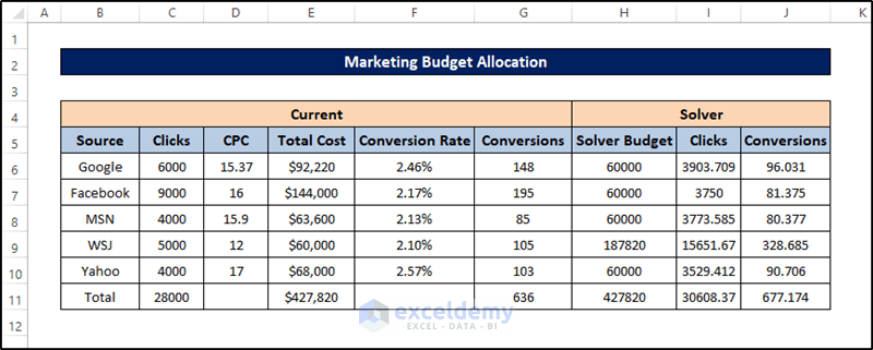
Example 6: Excel Solver for Marketing Budget Allocations

Finally, let’s take a look at a scenario where we need to use the solver in Excel for marketing budget allocations. For that, let’s take a dataset like this.

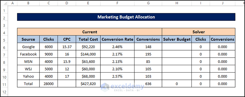
Here, we have the current stats on the left, and the portion where we are going to use the solver is on the right.

Follow these steps to find out how we can tackle this marketing problem with Excel Solver.

Steps:

• First, go to the Data tab on your ribbon and select the Solver from the Analysis group.

• Then write down the following constraints and the parameters as shown in the figure.

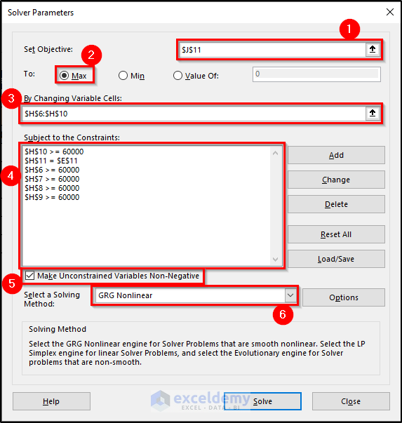
• After that, click on Solve.
• Next, click on OK on the Solver Results

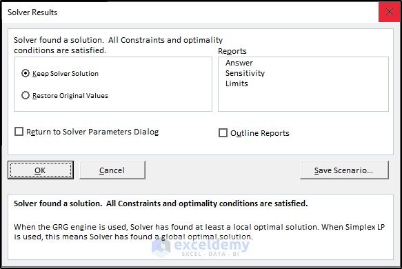
The values will change because of the constraints and parameters we have chosen.

You can use the solver in Excel in similar examples like that.

Read More: How to Use Excel Solver for Linear Programming

Download Practice Workbook

Download the workbook used for the demonstration from the link below.

Conclusion

That concludes the article for Excel solver examples. Hopefully, you have grasped the idea of using the Excel solver for different scenarios from these examples. I hope you found this guide helpful and informative. If you have any questions or suggestions, let us know in the comments below.

Excel Solver Examples: Knowledge Hub

<< Go Back to Solver in Excel | Learn Excel